
i3d::PMFilter< VOXELIN, VOXELOUT > Class Template Reference
[Image preprocessing filters]
This class implements together with class PMFilterFunction the Perona-Malik anisotropic diffusion filter, which was published by Perona and Malik. This filter was historical first published anisotropic diffusion filter and therefore is fundamental. As the other anisotropic filters, this filter smooths the image in the relatively continuos region and do not smooth the significante edges. In the typical output image is suppresed the noise and the edges remain sharp and well localised. The diffused image is the solution of the equation  . The particular implemantion is based on explicit finite difference solver and therefore there exist some limitations to the time step. If you want to use the schema with no timestep limitation take a look to the documentation of AOSPMFilter.
More...
. The particular implemantion is based on explicit finite difference solver and therefore there exist some limitations to the time step. If you want to use the schema with no timestep limitation take a look to the documentation of AOSPMFilter.
More...
#include <LevelSet.h>
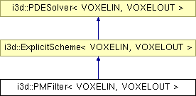
Inheritance diagram for i3d::PMFilter< VOXELIN, VOXELOUT >:
Public Member Functions | |
| int | SetNorm (int type) |
| Set the norm function. Possible values are ORIGINALPM, ALTERNATIVEPM and TUKEY. | |
| void | SetConductance (VOXELOUT c) |
Set the  conductance parameter. conductance parameter. | |
| VOXELOUT | GetConductance () |
| Get the conductance parameter. | |
Detailed Description
template<class VOXELIN, class VOXELOUT>
class i3d::PMFilter< VOXELIN, VOXELOUT >
This class implements together with class PMFilterFunction the Perona-Malik anisotropic diffusion filter, which was published by Perona and Malik. This filter was historical first published anisotropic diffusion filter and therefore is fundamental. As the other anisotropic filters, this filter smooths the image in the relatively continuos region and do not smooth the significante edges. In the typical output image is suppresed the noise and the edges remain sharp and well localised. The diffused image is the solution of the equation . The particular implemantion is based on explicit finite difference solver and therefore there exist some limitations to the time step. If you want to use the schema with no timestep limitation take a look to the documentation of AOSPMFilter.
The Perona Malik Filter is the historical first anisotropic diffusion filter. The image is smoothed by finding solution of partial differential equation
![\[ u_t = \mathrm{div} (g(|\nabla u|) \nabla u) \]](form_67.png)
where  is decreasing function of the image gradient, and
  is the input image (boundary condition of the PDE). The idea of this equation is to smooth the image in regions with almost no gradient and do not diffuse the image near significant edges. The strength of the diffusion is controled by the diffusivity function g. The diffusivity g is in original work of Perona and Malik computed by:
![\[ g(s) = \frac{1}{1+\left(\frac{s}{ \lambda}\right )^2} \]](form_68.png)
Perona and Malik considered also an alternative diffusion function:
![\[ g(s) = \mathrm{exp}(-(s/\lambda)^2) \]](form_69.png)
An consequently Black, Sapiro, Marimont, Heeger proposed the usage of Tukey Biweight norm:
![\[ \begin{array}[b]{l} g(s) = [1 - (2(s/\lambda))^2]^2 \quad |s| \le \lambda/\sqrt{2} \\ g(s) = 0 \quad \rm{otherwise} \\ \end{array} \]](form_81.png)
See the image bellow, there are displayed all three norms. The meaning of those norms is following: All three enables the diffusion on pixels with the gradient lower than . All three stops the diffusion on pixels with image gradient higher than  , but they differ on the strictness of the stopping.

Diffusivity g function: lambda = 5.0, left: original PM norm, middle: alternative PM Norm, right: Tukey Biweight Norm
between 1 and 10.All three norms can be used to produce meaningfull output.
A few of iterations (1 to 10) should be sufficient to to smooth the image. due to the limitation of used explicit numerical discretisation should be the time step lower than 0.25 for 2D images and lower than 0.125 for 3D images (See also the example code). If there is no time step set, the possible largest is set automatically.
The numerical scheme which finds the solution of the equation is implemented in ExplicitScheme class. This class inherits the solution.
The implementation of this class is based on the articles
Pietro Perona and Jitendra Malik, Scale-Space and Edge Detection Using Anisotropic Diffusion IEEE Transactions on Pattern Analysis and Machine Intelligence. Vol. 12. No. 7. July 1990. Michael J. Black, Guilermo Sapiro, David H. Marimont, David Heeger, Robust Anisotropic Diffusion , IEEE Transactions on Image Processing, Vol. 7. No. 3. March 1998 The example code uses the AOS implementation of PM diffusion filter.
   .....

   Image3d<GRAY8> i;
   Image3d<float> fimg;
   i.ReadImage('input.tif'); // read input image
   PMFilter<GRAY8,float> PM(i,fimg); // instantiate  the filter  (the two parameters are the input and the output image)
   PM.SetMaximumNumberOfIterations(3); // Set the number of iterations to 2
   PM.SetSpacing(1.0,1.0,2.0); // Set the spacing of spatial discretisation to 1,1,2
   PM.SetConductance(3.0); // Set the conductance parameter to 3.0
   PM.SetNorm(ORIGINALPM); // Set norm to original PM norm
   PM.Execute(); // Perform the work of the filter
   FloatToGray8NoWeight(fimg,i); //Convert the output float image to gray8 image
   i.SaveImage('output.tif'); // save the output of the filter

   ......
- Date:
- 2005
The documentation for this class was generated from the following files:
- LevelSet.h
- LevelSet.cc